- Retrieving Data
- Column Expressions
- Updating Data
- Subqueries
- Joins
- Aggregations
1. Retrieving Data
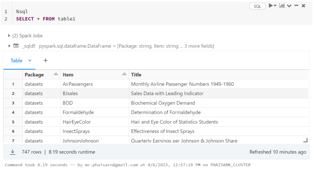
SELECT
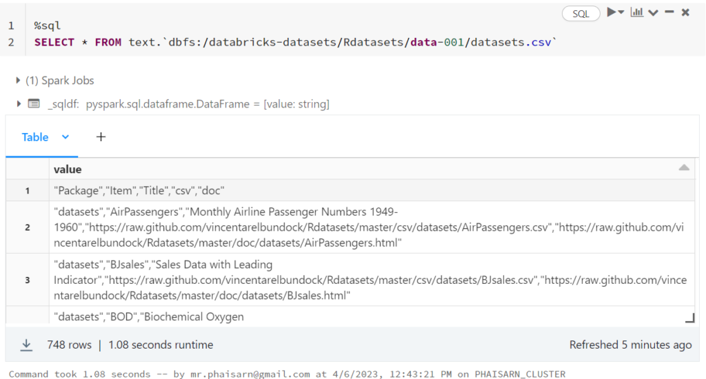
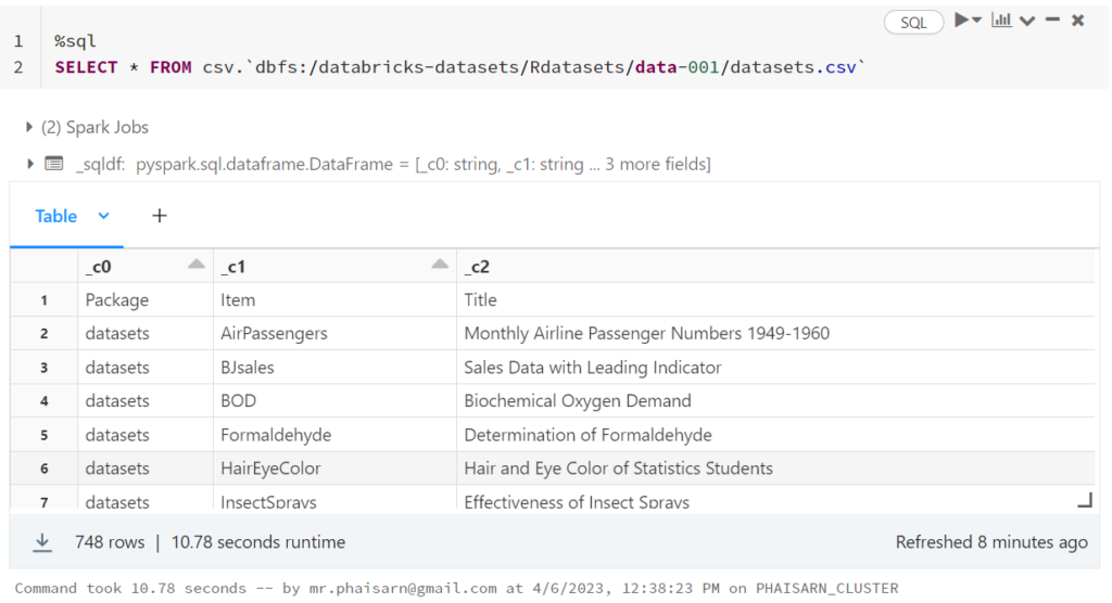
This simple command retrieves data from a table. The “*” represents “Select All,” so the command is selecting all data from the table
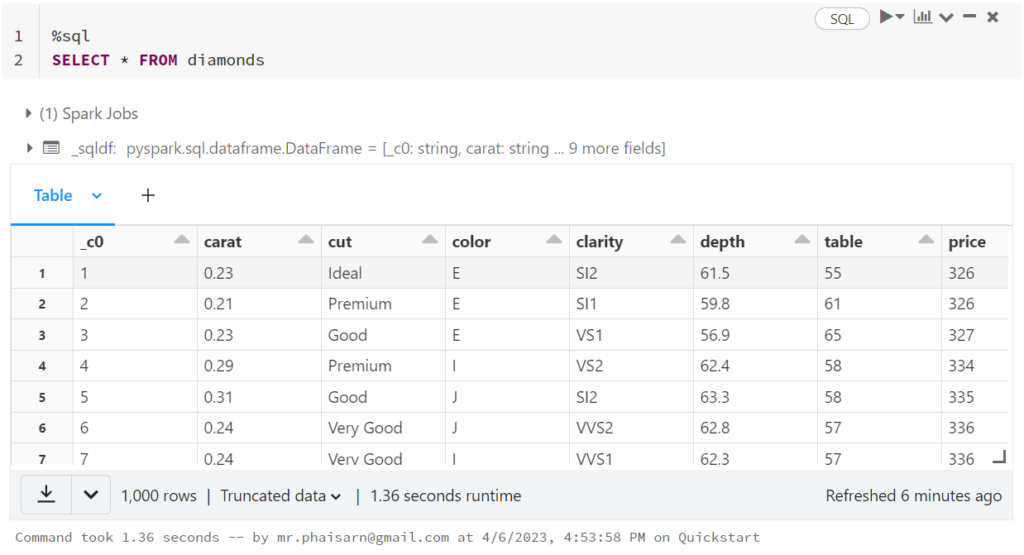
However, note that only 1,000 rows were retrieved. Databricks SQL defaults to only retrieving 1,000 rows from a table. If you wish to retrieve more, deselect the checkbox “LIMIT 1000”.
USE demo;
SELECT * FROM customers;
SELECT … AS
By adding the AS keyword, we can change the name of the column in the results.
Note that the column customer_name has been renamed Customer
USE demo;
SELECT customer_name AS Customer
FROM customers;
DISTINCT
If we add the DISTINCT keyword, we can ensure that we do not repeat data in the table.
There are more than 1,000 records that have a state in the state field. But, we only see 51 results because there are only 51 distinct state names.
USE demo;
SELECT DISTINCT state FROM customers;
WHERE
The WHERE keyword allows us to filter the data.
We are selecting from the customers table, but we are limiting the results to those customers who have a loyalty_segment of 3.
USE demo;
SELECT * FROM customers WHERE loyalty_segment = 3;
GROUP BY
We can run a simple COUNT aggregation by adding count() and GROUP BY to our query.
GROUP BY requires an aggregating function. We will discuss more aggregations later on.
USE demo;
SELECT loyalty_segment, count(loyalty_segment)
FROM customers
GROUP BY loyalty_segment;
ORDER BY
By adding ORDER BY to the query we just ran, we can place the results in a specific order.
ORDER BY defaults to ordering in ascending order. We can change the order to descending by adding DESC after the ORDER BY clause.
USE demo;
SELECT loyalty_segment, count(loyalty_segment)
FROM customers
GROUP BY loyalty_segment
ORDER BY loyalty_segment;
2. Column Expressions
Mathematical Expressions of Two Columns
In our queries, we can run calculations on the data in our tables. This can range from simple mathematical calculations to more complex computations involving built-in functions.
The results show that the Calculated Discount, the one we generated using Column Expressions, matches the Discounted Price.
USE demo;
SELECT sales_price - sales_price * promo_disc AS Calculated_Discount,
discounted_price AS Discounted_Price
FROM promo_prices;
Built-In Functions — String Column Manipulation
There are many, many Built-In Functions. We are going to talk about just a handful, so you can get a feel for how they work.
We are going to use a built-in function called lower(). This function takes a string expression and returns the same expression with all characters changed to lowercase. Let’s have a look.
USE demo;
SELECT lower(city) AS City
FROM customers;
Although the letters are now all lowercase, they are not the way the need to be. We want to have the first letter of each word capitalized.
USE demo;
SELECT initcap(city) AS City
FROM customers;
Date Functions
We want to use a function to make the date more human-readable. Let’s use from_unixtime().
The date looks better, but let’s adjust the formatting. Formatting options for many of the date and time functions are available here.
USE demo;
SELECT from_unixtime(promo_began, 'd MMM, y') AS Beginning_Date
FROM promo_prices;
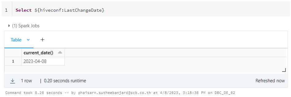
Date Calculations
In this code, we are using the function current_date() to get today’s date. We are then nesting from_unixtime() inside to_date in order to convert promo_began to a date object. We can then run the calculation.
USE demo;
SELECT current_date() - to_date(from_unixtime(promo_began)) FROM promo_prices;
CASE … WHEN
Often, it is important for us to use conditional logic in our queries. CASE … WHEN provides us this ability.
This statement allows us to change numeric values that represent loyalty segments into human-readable strings. It is certainly true that this association would more-likely occur using a join on two tables, but we can still see the logic behind CASE … WHEN
USE demo;
SELECT customer_name, loyalty_segment,
    CASE
        WHEN loyalty_segment = 0 THEN 'Rare'
        WHEN loyalty_segment = 1 THEN 'Occasional'
        WHEN loyalty_segment = 2 THEN 'Frequent'
        WHEN loyalty_segment = 3 THEN 'Daily'
    END AS Loyalty
FROM customers;
3. Updating Data
UPDATE
Let’s make those changes.
The UPDATE does exactly what it sounds like: It updates the table based on the criteria specified.
USE demo;
UPDATE customers SET city = initcap(lower(city));

SELECT city FROM customers;
INSERT INTO
In addition to updating data, we can insert new data into the table.
INSERT INTO is a command for inserting data into a table.
USE demo;
INSERT INTO loyalty_segments
    (loyalty_segment_id, loyalty_segment_description, unit_threshold, valid_from, valid_to)
VALUES
    (4, 'level_4', 100, current_date(), Null);

SELECT * FROM loyalty_segments;
INSERT TABLE
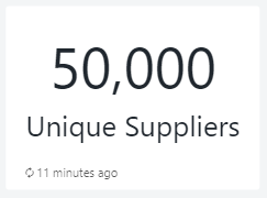
INSERT TABLE is a command for inserting entire tables into other tables. There are two tables suppliers and source_suppliers that currently have the exact same data.
After selecting from the table again, we note that the number of rows has doubled. This is because INSERT TABLE inserts all data in the source table, whether or not there are duplicates.
USE demo;
INSERT INTO suppliers TABLE source_suppliers;

SELECT * FROM suppliers;
INSERT OVERWRITE
If we want to completely replace the contents of a table, we can use INSERT OVERWRITE.
After running INSERT OVERWRITE and then retrieving a count(*) from the table, we see that we are back to the original count of rows in the table. INSERT OVERWRITE has replaced all the rows.
USE demo;
INSERT OVERWRITE suppliers TABLE source_suppliers;
SELECT * FROM suppliers;
4. Subqueries
Let’s create two new tables.
These two command use subqueries to SELECT from the customers table using specific criteria. The results are then fed into CREATE OR REPLACE TABLE and CREATE OR REPLACE TABLE statements. Incidentally, this type of statement is often called a CTAS statement for CREATE OR REPLACE TABLE … AS.
USE demo;
CREATE OR REPLACE TABLE high_loyalty_customers AS
    SELECT * FROM customers WHERE loyalty_segment = 3;
CREATE OR REPLACE TABLE low_loyalty_customers AS
    SELECT * FROM customers WHERE loyalty_segment = 1;
5. Joins
We are now going to run a couple of JOIN queries. The first is the most common JOIN, an INNER JOIN. Since INNER JOIN is the default, we can just write JOIN.
In this statement, we are joining the customers table and the loyalty_segments tables. When the loyalty_segment from the customers table matches the loyalty_segment_id from the loyalty_segments table, the rows are combined. We are then able to view the customer_name, loyalty_segment_description, and unit_threshold from both tables.
USE demo;
SELECT
    customer_name,
    loyalty_segment_description,
    unit_threshold
FROM customers
INNER JOIN loyalty_segments
ON customers.loyalty_segment = loyalty_segments.loyalty_segment_id;
CROSS JOIN
Even though the CROSS JOIN isn’t used very often, I wanted to demonstrate it.
First of all, note the use of UNION ALL. All this does is combine the results of all three queries, so we can view them all in one results set. The Customers row shows the count of rows in the customers table. Likewise, the Sales row shows the count of the sales table. Crossed shows the number of rows after performing the CROSS JOIN.
USE demo;
SELECT "Sales", count(*) FROM sales
UNION ALL
SELECT "Customers", count(*) FROM customers
UNION ALL
SELECT "Crossed", count(*) FROM customers
  CROSS JOIN sales;
6. Aggregations
Now, let’s move into aggregations. There are many aggregating functions you can use in your queries. Here are just a handful.
Again, we are viewing the results of a handful of queries using a UNION ALL.
USE demo;
SELECT "Sum" Function_Name, sum(units_purchased) AS Value
FROM customers
WHERE state = 'CA'
UNION ALL
SELECT "Min", min(discounted_price) AS Lowest_Discounted_Price
FROM promo_prices
UNION ALL
SELECT "Max", max(discounted_price) AS Highest_Discounted_Price
FROM promo_prices
UNION ALL
SELECT "Avg", avg(total_price) AS Mean_Total_Price
FROM sales
UNION ALL
SELECT "Standard Deviation", std(total_price) AS SD_Total_Price
FROM sales
UNION ALL
SELECT "Variance", variance(total_price) AS Variance_Total_Price
FROM sales;