Pandoc

If you need to convert files from one markup format into another, pandoc is your swiss-army knife.

Installing pandoc

The simplest way to get the latest pandoc release is to use the installer.

Download the latest installer for Windows (64-bit)

Demos – Try pandoc online

Try pandoc online!

Example

Getting started with pandoc

On Windows, you can use either the classic command prompt or the more modern PowerShell terminal. If you use Windows in desktop mode, run the cmd or powershell command from the Start menu. If you use the Windows 8 start screen instead, simply type cmd or powershell, and then run either the “Command Prompt” or “Windows Powershell” application. If you are using cmd, type chcp 65001 before using pandoc, to set the encoding to UTF-8.

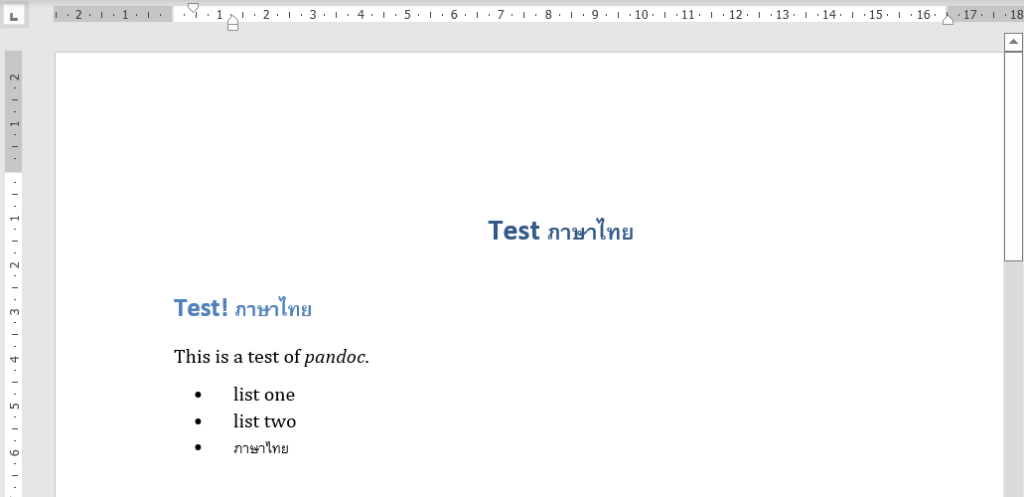
สร้างตัวอย่างไฟล์ test1.md

---
title: Test ภาษาไทย
...

# Test! ภาษาไทย

This is a test of *pandoc*.

- list one
- list two
- ภาษาไทย

รันคำสั่งที่ PowerShell

> pandoc test1.md -f markdown -t docx -s -o test1.docx

Pandoc User’s Guide

Ref

Table

1. เตรียมตารางด้วย SQL

สร้างตารางตัวอย่างชื่อ table_name (เป็น managed table)

%sql 
CREATE OR REPLACE TABLE table_name (
  id BIGINT GENERATED ALWAYS AS IDENTITY (START WITH 1 INCREMENT BY 1),
  name STRING,
  age INT,
  flag BOOLEAN,
  timestamp TIMESTAMP
)

คำสั่งต่างๆที่เกี่ยวข้องกับตาราง

%sql
SHOW CREATE TABLE table_name
%sql
DESCRIBE TABLE table_name
%sql
DESCRIBE HISTORY table_name

เพิ่มข้อมูลลงตาราง table_name (ที่ timestamp บวกเวลาไป 7 ชั่วโมง)

%sql
INSERT INTO
  table_name (name, age, flag, timestamp)
VALUES(
    'jack',
    '18',
    false,
    TIMESTAMPADD(HOUR, + 7, CURRENT_TIMESTAMP())
  )

ดูข้อมูลตาราง table_name

%sql
SELECT
  *
FROM
  table_name

หรือดูด้วย Delta Time Travel

%sql
SELECT
  *
FROM
  table_name VERSION AS OF 1
+----+------+-----+-------+------------------------------+
| id | name | age | flag  | timestamp                    |
+----+------+-----+-------+------------------------------+
| 1  | jack | 18  | false | 2022-09-07T16:29:05.071+0000 |
| 2  | tip  | 14  | false | 2022-09-07T17:17:00.285+0000 |
+----+------+-----+-------+------------------------------+

ลบตาราง table_name

%sql
DROP TABLE table_name

2. Spark SQL (Python)

เตรียมคิวรี

%python
query = """
SELECT * 
FROM   table_name
"""

รันคิวรี

%python
df = spark.sql(query)

ดู schema

%python
df.printSchema()
root
 |-- id: long (nullable = true)
 |-- name: string (nullable = true)
 |-- age: integer (nullable = true)
 |-- flag: boolean (nullable = true)
 |-- timestamp: timestamp (nullable = true)
%python
print(df)
DataFrame[id: bigint, name: string, age: int, flag: boolean, timestamp: timestamp]

ดูข้อมูล

%python
display(df)
+----+------+-----+-------+------------------------------+
| id | name | age | flag  | timestamp                    |
+----+------+-----+-------+------------------------------+
| 1  | jack | 18  | false | 2022-09-07T16:29:05.071+0000 |
| 2  | tip  | 14  | false | 2022-09-07T17:17:00.285+0000 |
+----+------+-----+-------+------------------------------+
%python
df.show()
+---+----+---+-----+--------------------+
| id|name|age| flag|           timestamp|
+---+----+---+-----+--------------------+
|  1|jack| 18|false|2022-09-07 17:10:...|
|  2| tip| 14|false|2022-09-07 17:17:...|
+---+----+---+-----+--------------------+
%python
# Select only the "name" column
df.select("name").show()
+----+
|name|
+----+
|jack|
| tip|
+----+
%python
# Select everybody, but increment the age by 1
df.select(df['name'], df['age'] + 1).show()
+----+---------+
|name|(age + 1)|
+----+---------+
|jack|       19|
| tip|       15|
+----+---------+
%python
# Select people older than 15
df.filter(df['age'] > 15).show()
+---+----+---+-----+--------------------+
| id|name|age| flag|           timestamp|
+---+----+---+-----+--------------------+
|  1|jack| 18|false|2022-09-07 17:10:...|
+---+----+---+-----+--------------------+
%python
# Count people by age
df.groupBy("age").count().show()
+---+-----+
|age|count|
+---+-----+
| 18|    1|
| 14|    1|
+---+-----+
%python
print(type(df.collect()))
df.collect()
[Row(id=1, name='jack', age=18, flag=False, timestamp=datetime.datetime(2022, 9, 7, 17, 10, 34, 193000)),
 Row(id=2, name='tip', age=14, flag=False, timestamp=datetime.datetime(2022, 9, 7, 17, 17, 0, 285000))]
%python
for row in df.collect():
  print(row['name'])
jack
tip

Query firebase_screen

screen_view (event_params)

  • firebase_screen
  • firebase_screen_class
  • firebase_screen_id (int_value)
  • firebase_previous_screen
  • firebase_previous_class
  • firebase_previous_id (int_value)
  • engagement_time_msec
  • ga_session_id (int_value)
  • ga_session_number (int_value)
SELECT
  user_pseudo_id,
  (SELECT value.int_value    FROM UNNEST(event_params) WHERE key = 'ga_session_id')            AS ga_session_id,
  (SELECT value.int_value    FROM UNNEST(event_params) WHERE key = 'firebase_previous_id')     AS firebase_previous_id,
  (SELECT value.int_value    FROM UNNEST(event_params) WHERE key = 'firebase_screen_id')       AS firebase_screen_id,
  (SELECT value.string_value FROM UNNEST(event_params) WHERE key = 'firebase_previous_screen') AS firebase_previous_screen,
  (SELECT value.string_value FROM UNNEST(event_params) WHERE key = 'firebase_screen')          AS firebase_screen,
  (SELECT value.string_value FROM UNNEST(event_params) WHERE key = 'firebase_previous_class')  AS firebase_previous_class,
  (SELECT value.string_value FROM UNNEST(event_params) WHERE key = 'firebase_screen_class')    AS firebase_screen_class,
FROM
  `my_project.my_dataset.events_*`
WHERE
  event_name = 'screen_view'
  AND _TABLE_SUFFIX BETWEEN '20220901' AND '20220901'
ORDER BY 
  ga_session_id,
  event_timestamp

firebase_previous_screen และ firebase_screen

แสดงทุก screen , แสดงคู่ firebase_previous_screen และ firebase_screen

SELECT
  firebase_previous_screen,
  firebase_screen,
  COUNT(*) AS cnt
FROM 
(
  SELECT
    (SELECT value.string_value FROM UNNEST(event_params) WHERE key = 'firebase_previous_screen') AS firebase_previous_screen,
    (SELECT value.string_value FROM UNNEST(event_params) WHERE key = 'firebase_screen') AS firebase_screen,
  FROM
    `my_project.my_dataset.events_*`
  WHERE
    event_name = 'screen_view'
    AND _TABLE_SUFFIX BETWEEN '20220901' AND '20220901'
)
GROUP BY 
  firebase_previous_screen,
  firebase_screen
ORDER BY 
  firebase_screen
+--------------------------+-----------------+-----+
| firebase_previous_screen | firebase_screen | cnt |
+--------------------------+-----------------+-----+
| ScreenA                  | ScreenB         | 10  |
| ScreenB                  | ScreenC         | 5   |
| ScreenD                  | ScreenE         | 1   |
+--------------------------+-----------------+-----+

เลือกเฉพาะ screen จาก session ที่มี screen ที่กำหนดเท่านั้น (เช่น ใน session นั้นๆมี ‘ScreenA’ หรือ ‘ScreenB’ ก็แสดงทุก screen ใน session นั้น)

WITH table_screen_view AS
(
  SELECT
    user_pseudo_id,
    event_timestamp,
    (SELECT value.int_value FROM UNNEST(event_params) WHERE key = 'ga_session_id') AS ga_session_id,
    (SELECT value.string_value FROM UNNEST(event_params) WHERE key = 'firebase_previous_screen') AS firebase_previous_screen,
    (SELECT value.string_value FROM UNNEST(event_params) WHERE key = 'firebase_screen') AS firebase_screen,
  FROM
    `my_project.my_dataset.events_*`
  WHERE
    event_name = 'screen_view'
    AND _TABLE_SUFFIX BETWEEN '20220901' AND '20220901'
)
SELECT 
  firebase_previous_screen,
  firebase_screen,
  COUNT(*) AS cnt,
FROM table_screen_view
WHERE 
  ga_session_id IN ( SELECT ga_session_id 
                     FROM table_screen_view 
                     WHERE firebase_screen IN ('ScreenA', 'ScreenB')
                   )
GROUP BY
  firebase_previous_screen,
  firebase_screen
ORDER BY 
  firebase_screen
+--------------------------+-----------------+-----+
| firebase_previous_screen | firebase_screen | cnt |
+--------------------------+-----------------+-----+
| ScreenA                  | ScreenB         | 10  |
| ScreenB                  | ScreenC         | 5   |
+--------------------------+-----------------+-----+

firebase_screen

แสดงทุก screen (firebase_screen) ใน session เดียวกัน โดยเรียงจาก event_timestamp

WITH sequence_screen AS
(
  SELECT 
    ga_session_id,
    firebase_screen,
    concat('stage', cast(stage_rank as string)) AS stage_rank,
  FROM
  (
    SELECT 
      ga_session_id,
      firebase_screen,
      RANK() OVER (PARTITION BY ga_session_id ORDER BY event_timestamp ASC) AS stage_rank,
    FROM
    (
      SELECT
        event_timestamp,
        (SELECT value.int_value FROM UNNEST(event_params) WHERE key = 'ga_session_id') AS ga_session_id,
        (SELECT value.string_value FROM UNNEST(event_params) WHERE key = 'firebase_screen') AS firebase_screen,
      FROM
        `my_project.my_dataset.events_*`
      WHERE
        event_name = 'screen_view'
        AND _TABLE_SUFFIX BETWEEN '20220901' AND '20220901'
    )
  )  
)
SELECT * FROM sequence_screen 
PIVOT(any_value(firebase_screen) FOR stage_rank IN ('stage1', 'stage2', 'stage3', 'stage4', 'stage5'))
ORDER BY ga_session_id
+-------------------------+---------+---------+---------+---------+
| ga_session_id | stage1  | stage2  | stage3  | stage4  | stage5  |
+-------------------------+---------+---------+---------+---------+
| 1234567891    | ScreenA | ScreenB | ScreenC | ScreenD | ScreenE |
| 1234567892    | ScreenA | ScreenC | ScreenD | NULL    | NULL    |
+-------------------------+---------+---------+---------+---------+

Query multiple tables

Wildcard tables enable you to query multiple tables using concise SQL statements. Wildcard tables are available only in standard SQL. For equivalent functionality in legacy SQL, see Table wildcard functions.

A wildcard table represents a union of all the tables that match the wildcard expression.

# Standard SQL
SELECT * 
FROM `my_project.my_dataset.my_table_202208*`

Each row in the wildcard table contains a special column, _TABLE_SUFFIX, which contains the value matched by the wildcard character.

For information on wildcard table syntax, see Wildcard tables in the standard SQL reference.

# Standard SQL
SELECT * 
FROM `my_project.my_dataset.my_table_*`
WHERE _TABLE_SUFFIX BETWEEN '20220801' AND '20220831'

BigQuery – Rank

RANK()
OVER over_clause

over_clause:
  { named_window | ( [ window_specification ] ) }

window_specification:
  [ named_window ]
  [ PARTITION BY partition_expression [, ...] ]
  ORDER BY expression [ { ASC | DESC }  ] [, ...]

Example1

WITH Numbers AS
 (SELECT 1 as x
  UNION ALL SELECT 2
  UNION ALL SELECT 2
  UNION ALL SELECT 5
  UNION ALL SELECT 8
  UNION ALL SELECT 10
  UNION ALL SELECT 10
)
SELECT x,
  RANK() OVER (ORDER BY x ASC) AS rank
FROM Numbers
+-------------------------+
| x          | rank       |
+-------------------------+
| 1          | 1          |
| 2          | 2          |
| 2          | 2          |
| 5          | 4          |
| 8          | 5          |
| 10         | 6          |
| 10         | 6          |
+-------------------------+

Example2

WITH finishers AS
 (SELECT 'Sophia Liu' as name,
  TIMESTAMP '2016-10-18 2:51:45' as finish_time,
  'F30-34' as division
  UNION ALL SELECT 'Lisa Stelzner', TIMESTAMP '2016-10-18 2:54:11', 'F35-39'
  UNION ALL SELECT 'Nikki Leith', TIMESTAMP '2016-10-18 2:59:01', 'F30-34'
  UNION ALL SELECT 'Lauren Matthews', TIMESTAMP '2016-10-18 3:01:17', 'F35-39'
  UNION ALL SELECT 'Desiree Berry', TIMESTAMP '2016-10-18 3:05:42', 'F35-39'
  UNION ALL SELECT 'Suzy Slane', TIMESTAMP '2016-10-18 3:06:24', 'F35-39'
  UNION ALL SELECT 'Jen Edwards', TIMESTAMP '2016-10-18 3:06:36', 'F30-34'
  UNION ALL SELECT 'Meghan Lederer', TIMESTAMP '2016-10-18 2:59:01', 'F30-34')
SELECT name,
  finish_time,
  division,
  RANK() OVER (PARTITION BY division ORDER BY finish_time ASC) AS finish_rank
FROM finishers;
+-----------------+------------------------+----------+-------------+
| name            | finish_time            | division | finish_rank |
+-----------------+------------------------+----------+-------------+
| Sophia Liu      | 2016-10-18 09:51:45+00 | F30-34   | 1           |
| Meghan Lederer  | 2016-10-18 09:59:01+00 | F30-34   | 2           |
| Nikki Leith     | 2016-10-18 09:59:01+00 | F30-34   | 2           |
| Jen Edwards     | 2016-10-18 10:06:36+00 | F30-34   | 4           |
| Lisa Stelzner   | 2016-10-18 09:54:11+00 | F35-39   | 1           |
| Lauren Matthews | 2016-10-18 10:01:17+00 | F35-39   | 2           |
| Desiree Berry   | 2016-10-18 10:05:42+00 | F35-39   | 3           |
| Suzy Slane      | 2016-10-18 10:06:24+00 | F35-39   | 4           |
+-----------------+------------------------+----------+-------------+

BigQuery – Rotates columns into rows

FROM from_item[, ...] unpivot_operator

unpivot_operator:
    UNPIVOT [ { INCLUDE NULLS | EXCLUDE NULLS } ] (
        { single_column_unpivot | multi_column_unpivot }
    ) [unpivot_alias]

single_column_unpivot:
    values_column
    FOR name_column
    IN (columns_to_unpivot)

multi_column_unpivot:
    values_column_set
    FOR name_column
    IN (column_sets_to_unpivot)

values_column_set:
    (values_column[, ...])

columns_to_unpivot:
    unpivot_column [row_value_alias][, ...]

column_sets_to_unpivot:
    (unpivot_column [row_value_alias][, ...])

unpivot_alias and row_value_alias:
    [AS] alias

The UNPIVOT operator rotates columns into rows. UNPIVOT is part of the FROM clause.

  • UNPIVOT can be used to modify any table expression.
  • Combining UNPIVOT with FOR SYSTEM_TIME AS OF is not allowed, although users may use UNPIVOT against a subquery input which itself uses FOR SYSTEM_TIME AS OF.
  • WITH OFFSET clause immediately preceding the UNPIVOT operator is not allowed.
  • PIVOT aggregations cannot be reversed with UNPIVOT.
WITH Produce AS (
  SELECT 'Kale' as product, 51 as Q1, 23 as Q2, 45 as Q3, 3 as Q4 UNION ALL
  SELECT 'Apple', 77, 0, 25, 2)
SELECT * FROM Produce
+---------+----+----+----+----+
| product | Q1 | Q2 | Q3 | Q4 |
+---------+----+----+----+----+
| Kale    | 51 | 23 | 45 | 3  |
| Apple   | 77 | 0  | 25 | 2  |
+---------+----+----+----+----+
SELECT * FROM Produce
UNPIVOT(sales FOR quarter IN (Q1, Q2, Q3, Q4))
+---------+-------+---------+
| product | sales | quarter |
+---------+-------+---------+
| Kale    | 51    | Q1      |
| Kale    | 23    | Q2      |
| Kale    | 45    | Q3      |
| Kale    | 3     | Q4      |
| Apple   | 77    | Q1      |
| Apple   | 0     | Q2      |
| Apple   | 25    | Q3      |
| Apple   | 2     | Q4      |
+---------+-------+---------+

BigQuery – Rotates rows into columns

Transforming BigQuery Rows to Columns

The Pivot operation in Google BigQuery changes rows into columns by using Aggregation. Let’s understand the working of the Pivot operator with the help of a table containing information about Products and their Sales per Quarter. The following examples reference a table called Produce that looks like this before applying the Pivot operation:

Example1

WITH Produce AS (
  SELECT 'Win' as product, 51 as sales, 'Q1' as quarter UNION ALL
  SELECT 'Win', 23, 'Q2' UNION ALL
  SELECT 'Win', 45, 'Q3' UNION ALL
  SELECT 'Win', 3, 'Q4' UNION ALL
  SELECT 'Linux', 77, 'Q1' UNION ALL
  SELECT 'Linux', 0, 'Q2' UNION ALL
  SELECT 'Linux', 25, 'Q3' UNION ALL
  SELECT 'Linux', 2, 'Q4')
SELECT * FROM Produce
+---------+-------+---------+
| product | sales | quarter |
+---------+-------+---------+
| Win     | 51    | Q1      |
| Win     | 23    | Q2      |
| Win     | 45    | Q3      |
| Win     | 3     | Q4      |
| Linux   | 77    | Q1      |
| Linux   | 0     | Q2      |
| Linux   | 25    | Q3      |
| Linux   | 2     | Q4      |
+---------+-------+---------+

After applying the Pivot operator, you can rotate the Sales and Quarter into Q1, Q2, Q3, and Q4 columns. This will make the table much more readable. The query for the same would look something like this:

SELECT * FROM
  (SELECT * FROM Produce)
  PIVOT(SUM(sales) FOR quarter IN ('Q1', 'Q2', 'Q3', 'Q4'))
+---------+----+----+----+----+
| product | Q1 | Q2 | Q3 | Q4 |
+---------+----+----+----+----+
| Win     | 51 | 23 | 45 | 3  |
| Linux   | 77 | 0  | 25 | 2  |
+---------+----+----+----+----+

Example2

WITH `table_name` AS (
  SELECT '1662104425' `ga_session_id`, 'page_a' AS `page`, 'r1' AS `rank` UNION ALL
  SELECT '1662104425', 'page_b', 'r2' UNION ALL
  SELECT '1662104425', 'page_c', 'r3' UNION ALL
  SELECT '1662104425', 'page_d', 'r4' UNION ALL
  SELECT '1662104425', 'page_e', 'r5' UNION ALL
  SELECT '1662091784', 'page_b', 'r1' UNION ALL
  SELECT '1662091784', 'page_c', 'r2' UNION ALL
  SELECT '1662091784', 'page_d', 'r3'
)  
SELECT * FROM table_name
Rowga_session_idpagerank
11662104425page_ar1
21662104425page_br2
31662104425page_cr3
41662104425page_dr4
51662104425page_er5
61662091784page_br1
71662091784page_cr2
81662091784page_dr3

ใช้ ANY_VALUE

SELECT * FROM table_name
PIVOT(any_value(page) FOR rank IN ('r1', 'r2', 'r3', 'r4', 'r5'))
Rowga_session_idr1r2r3r4r5
11662104425page_apage_bpage_cpage_dpage_e
21662091784page_bpage_cpage_dnullnull

Spark DataFrame

from pyspark.sql import SQLContext
sqlContext = SQLContext(sc)
sqlContext 

df  = sqlContext.sql("""
  SELECT *
  FROM   some_schema.some_table
  WHERE  eff_date >= '2022-05-01'
  AND    eff_date < '2022-06-01'
""")
print(type(df))
<class 'pyspark.sql.dataframe.DataFrame'>
data = [('A', "1"),
        ('B', "2"),
        ('C', "3"),
        ('D', "4"),
        ("Cate", "ID")
        ]
print(type(data))  # <class 'list'>
df = spark.createDataFrame(data)
print(type(df))    # <class 'pyspark.sql.dataframe.DataFrame'>
data = [{"Category": 'A', "ID": 1, "Value": 121.44, "Truth": True},
        {"Category": 'B', "ID": 2, "Value": 300.01, "Truth": False},
        {"Category": 'C', "ID": 3, "Value": 10.99, "Truth": None},
        {"Category": 'D', "ID": 4, "Value": 33.87, "Truth": True}
        ]
print(type(data))  # <class 'list'>
df = spark.createDataFrame(data)
print(type(df))    # <class 'pyspark.sql.dataframe.DataFrame'>
li = df.collect()
print(type(li))    # <class 'list'>
print(li[0])
# Row(Category='A', ID=1, Truth=True, Value=121.44)

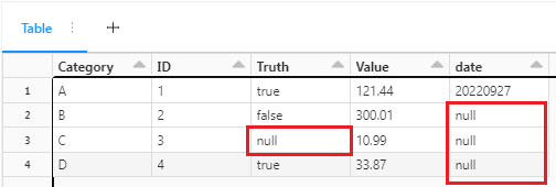
กำหนดค่าเป็น null ได้ด้วยการให้ค่า None หรือ ไม่ให้ค่าตัวแปรนั้น

data = [{"Category": 'A', "ID": 1, "Value": 121.44, "Truth": True, "date": "20220927"},
        {"Category": 'B', "ID": 2, "Value": 300.01, "Truth": False},
        {"Category": 'C', "ID": 3, "Value": 10.99, "Truth": None},
        {"Category": 'D', "ID": 4, "Value": 33.87, "Truth": True}
        ]
print(type(data))     # <class 'list'>
print(type(data[0]))  # <class 'dict'>
df = spark.createDataFrame(data)
display(df)

Pyspark add new row to dataframe

create 1st dataframe

%python
columns = ['Identifier', 'Value', 'Extra Discount']
vals = [(1, 150, 0), (2, 160, 12)]
df = spark.createDataFrame(vals, columns)
df.show()
+----------+-----+--------------+
|Identifier|Value|Extra Discount|
+----------+-----+--------------+
|         1|  150|             0|
|         2|  160|            12|
+----------+-----+--------------+

create 2nd dataframe

%python
newRow = spark.createDataFrame([(3,205,7)], columns)
newRow.show()
+----------+-----+--------------+
|Identifier|Value|Extra Discount|
+----------+-----+--------------+
|         3|  205|             7|
+----------+-----+--------------+

union dataframe

%python
new_df = df.union(newRow)
new_df.show()
+----------+-----+--------------+
|Identifier|Value|Extra Discount|
+----------+-----+--------------+
|         1|  150|             0|
|         2|  160|            12|
|         3|  205|             7|
+----------+-----+--------------+

Merge pandas dataFrame

create dataframe

%python
import pyspark.pandas as ps
df1 = ps.DataFrame({'lkey': ['foo', 'bar', 'baz', 'foo'],
                    'value': [1, 2, 3, 5]},
                   columns=['lkey', 'value'])
display(df1)
#   lkey  value
# 0  foo      1
# 1  bar      2
# 2  baz      3
# 3  foo      5
# df2

df2 = ps.DataFrame({'rkey': ['foo', 'bar', 'baz', 'foo'],
                    'value': [5, 6, 7, 8]},
                   columns=['rkey', 'value'])
display(df2)
#   rkey  value
# 0  foo      5
# 1  bar      6
# 2  baz      7
# 3  foo      8

merge

%python
merged = df1.merge(df2, left_on='lkey', right_on='rkey')
display(merged)
#   lkey  value_x rkey  value_y
#    bar        2  bar        6
#    baz        3  baz        7
#    foo        1  foo        5
#    foo        1  foo        8
#    foo        5  foo        5
#    foo        5  foo        8

Using Spark to Write Data to a Single CSV File

Apache Spark is a system designed to work with very large datasets. Its default behavior reflects the assumption that you will be working with a large dataset that is split across many nodes in a cluster.

When you use Apache Spark to write a dataframe to disk, you will notice that it writes the data into multiple files. Let’s look at an example and see this in action.

# First, we just read in some sample data so we have a Spark dataframe
df = spark.read.option("header", "true").csv("dbfs:/databricks-datasets/atlas_higgs/atlas_higgs.csv")

# Now, let's write this data out in CSV format so we can see how Spark writes the files
df.write.format("csv").mode("overwrite").save("/my-output/default-csv")

Now let’s take a look at the CSV files that Spark wrote…

dbutils.fs.ls("/my-output/default-csv")
Out[22]: [FileInfo(path='dbfs:/my-output/default-csv/_SUCCESS', name='_SUCCESS', size=0),
 FileInfo(path='dbfs:/my-output/default-csv/_committed_3363429043923895909', name='_committed_3363429043923895909', size=1256),
 FileInfo(path='dbfs:/my-output/default-csv/_started_3363429043923895909', name='_started_3363429043923895909', size=0),
 FileInfo(path='dbfs:/my-output/default-csv/part-00000-tid-3363429043923895909-2caa68d8-1164-41ee-9c37-2bce95052501-31-1-c000.csv', name='part-00000-tid-3363429043923895909-2caa68d8-1164-41ee-9c37-2bce95052501-31-1-c000.csv', size=4193821),
 FileInfo(path='dbfs:/my-output/default-csv/part-00001-tid-3363429043923895909-2caa68d8-1164-41ee-9c37-2bce95052501-32-1-c000.csv', name='part-00001-tid-3363429043923895909-2caa68d8-1164-41ee-9c37-2bce95052501-32-1-c000.csv', size=4194469),
 FileInfo(path='dbfs:/my-output/default-csv/part-00002-tid-3363429043923895909-2caa68d8-1164-41ee-9c37-2bce95052501-33-1-c000.csv', name='part-00002-tid-3363429043923895909-2caa68d8-1164-41ee-9c37-2bce95052501-33-1-c000.csv', size=4194236),
 FileInfo(path='dbfs:/my-output/default-csv/part-00003-tid-3363429043923895909-2caa68d8-1164-41ee-9c37-2bce95052501-34-1-c000.csv', name='part-00003-tid-3363429043923895909-2caa68d8-1164-41ee-9c37-2bce95052501-34-1-c000.csv', size=4194352),
...

You will notice that our dataset was not written to one, single CSV file in a nice, tidy format. Instead, the rows are spread out across a bunch of different CSV files. Spark can work easily with these multiple files. However, if you want to share this data with other systems, having multiple files can be cumbersome.

Before we look at how to change Spark’s behavior, we need to understand why Spark writes the data this way.

The key thing to always remember about Spark is that the data is always spread out across multiple computers. The data doesn’t reside in the memory of just one computer. It has been divided into multiple partitions, and those partitions are distributed across many computers.

When you tell Spark to write your data, it completes this operation in parallel. The driver tells all of the nodes to start writing their data at the same time. So each node in the cluster starts writing all of the partitions that it has at the same time all of the other nodes are writing all of their partitions. Therefore, Spark can’t write the data to just one file because all of the nodes would be tripping over each other. They would each try to write to the same file and end up overwriting the data that other nodes had written.

To solve this problem, Spark saves the data from each partition to its own file. Therefore, the number of files that get written is equal to the number of partitions that Spark created for your data.

Changing Spark’s Behavior

While Spark is designed to work with large, mult-terabyte datasets that could never fit into the memory of just one computer, we sometimes use it to work with smaller datasets. And sometime this dataset is relatively small… just a couple of gigabytes or even a few hundred megabytes. If you find yourself working with a small dataset like this, you can get Spark to write the data to just one file.

That last point is very important and bears repeating. To make this work, all of the data must be loaded into the memory of just one computer. Therefore, this technique only works on small datasets. If the nodes in your cluster each have 16GB of RAM, then you can probably make this work with 10GB of data or less. If you have a dataset that is bigger than the amount of RAM on each node, you cannot use this technique because you will risk crashing your cluster.

Fortunately, our sample dataset above is less than 100MB. So, keeping in mind the important limitation described above, this dataset should easily fit in the memory of just one PC. So let’s proceed with writing out our dataset to just one CSV file. There are a couple of ways to achieve this, and we will look at both of them.

Option 1: Use the coalesce Feature

The Spark Dataframe API has a method called coalesce that tells Spark to shuffle your data into the specified number of partitions. Since our dataset is small, we use this to tell Spark to rearrange our data into a single partition before writing out the data.

Note, though, that there is a performance penalty for this. Before writing the data, Spark must shuffle the data from all of the nodes to a single partition on a single node. This takes time and puts traffic on the cluster’s network. For a ver small dataset (like the one here in our example), this is a small penalty, but it will increase as the size of your data increases.

df\
.coalesce(1)\
.write\
.format("csv")\
.mode("overwrite")\
.save("/my-output/coalesce-csv")

Let’s take a look at the files created by Spark after using the coalesce method.

dbutils.fs.ls("/my-output/coalesce-csv")
Out[27]: [FileInfo(path='dbfs:/my-output/coalesce-csv/_SUCCESS', name='_SUCCESS', size=0),
 FileInfo(path='dbfs:/my-output/coalesce-csv/_committed_8239842462067349322', name='_committed_8239842462067349322', size=112),
 FileInfo(path='dbfs:/my-output/coalesce-csv/_started_8239842462067349322', name='_started_8239842462067349322', size=0),
 FileInfo(path='dbfs:/my-output/coalesce-csv/part-00000-tid-8239842462067349322-52e5d421-3f6b-4768-a979-71ac9a0c9ee2-45-1-c000.csv', name='part-00000-tid-8239842462067349322-52e5d421-3f6b-4768-a979-71ac9a0c9ee2-45-1-c000.csv', size=55253165)]

You will notice that Spark still wrote the data into a directory, and that directory has multiple files. There are the Spark control files (e.g. the “SUCCESS” file, the “started” file, and the “committed” file). But there is only Cone SV file containing our data. Unfortunately, this file does not have a friendly name. If we want to share this file, we may want to rename it to something shorter. We can Python to clean up the control files and rename the data file.

data_location = "/my-output/coalesce-csv/"

files = dbutils.fs.ls(data_location)
csv_file = [x.path for x in files if x.path.endswith(".csv")][0]
dbutils.fs.mv(csv_file, data_location.rstrip('/') + ".csv")
dbutils.fs.rm(data_location, recurse = True)
Out[44]: True

Now let’s take one more look at our files to see that we have just one CSV file with a nice, friendly name.

dbutils.fs.ls("/my-output")
Out[45]: [FileInfo(path='dbfs:/my-output/coalesce-csv.csv', name='coalesce-csv.csv', size=55253165),
 FileInfo(path='dbfs:/my-output/default-csv/', name='default-csv/', size=0)]

Option 2: Use collect and Pandas

If you’ve used Python for data science work, you may be familiar with the pandas package. This popular tool allows you to create in-memory dataframes on a single computer. If your Spark dataframe is small enough to fit into the RAM of your cluster’s driver node, then you can simply convert your Spark dataframe to a pandas dataframe. Then you can use the standard pandas functionality to save your pandas dataframe to a single CSV file.

pd = df.toPandas()
pd.to_csv("/dbfs/my-output/pandas.csv")

And now if we look at our output directory, we will see our new CSV file.

dbutils.fs.ls("/my-output")
Out[52]: [FileInfo(path='dbfs:/my-output/coalesce-csv.csv', name='coalesce-csv.csv', size=55253165),
 FileInfo(path='dbfs:/my-output/default-csv/', name='default-csv/', size=0),
 FileInfo(path='dbfs:/my-output/pandas.csv', name='pandas.csv', size=56892564)]

That was super easy! But you must be very careful with this approach. It will only work with small datasets. If you try to convert a large dataframe to a pandas dataframe, you could crash the driver node of your cluster. Make sure your driver node has enough RAM to hold the entire dataset.

One other note on this approach. You will notice that throughout this notebook we have written data to the DBFS. We’ve done this using paths relative to the root of the DBFS, like: /my-output/coalesce-csv. In Databricks, Spark and the dbutils tool are all “DBFS-aware”. Whenever you supply a filepath to these tools, it assumes that you want to use the DBFS. Non-Spark tools (like the pandas tool) are not “DBFS-aware”. Whenever you give them a filepath, they assume you want to use the filesystem of the driver node. Therefore, you must add /dbfs/ to the beginning of your filepath so these tools will look in the right place. For example, when we used the to_csv method from the pandas package, we had to use /dbfs/my-output/pandas.csv as our location.